Super-resolution
DEM resolution can be increased with machine learning techniques.
Content
Input data
Data preprocessing for training
Test data
Types of Super-resolution algorithm
Previous attempts
VDSR-based super-resolution DEM
Keras Tuner
Next Steps
Publications and Implementations
Input data
Super-resolution (SR) machine learning techniques were developed based on well-known image datasets like DIV2K. These contain PNG images with three layers (RGB - red, green and blue) and 8-bit values (0-255).
This is not the case for DEMs, where we have one layer with float values, or at least 16 bit values. Common geodata formats such as GeoTIFF cannot be read out-of-the-box by the image libraries used in machine learning frameworks, and the code of most SR implementations therefore needs to be adjusted.
Have a look at this Jupyter Notebook to see how to handle GeoTIFF files with Tensorflow. Thanks to Zushicat for the support.
Furthermore, for most algorithms, downscale processing plays an important role:
"DIV2K bicubic downscaled images have been created with the MATLAB imresize function. It is important that you create downscaled versions of Set5 images in the very same way [...] For example, to bicubic downscale by a factor of 4 use imresize(x, 0.25, method='bicubic') and then feed the downscaled image into a pre-trained model" (source: krasserm/super-resolution).
The information in a high-resolution image is therefore partly available in each pixel of a downscaled image.
However, this is not realistic for SR DEMs. In many cases, we do not know exactly how a low-resolution DEM was derived from a high-resolution dataset. The nearest neighbours algorithm is the best case scenario, because the original values are preserved.
Let´s have a look at an example. The authorities in Bavaria (Germany) offer a range of different Digital Terrain products:
| Product | horizontal resolution [m] | height accuracy [m] | license |
| DGM 1 | 1 | generally better than +- 0.2 | proprietary |
| DGM 2 | 2 | generally better than +- 0.2 | proprietary |
| DGM 5 | 5 | generally better than +- 0.2 | proprietary |
| DGM 10 | 10 | generally better than +- 0.2 | proprietary |
| DGM 25 | 25 | ~ +- 2-3 | proprietary |
| DGM 50 | 50 | ~ +- 5 | CC BY 3.0 DE |
Tab. 1: DTM (DGM in German) data products from Bavaria (link).
From the test data of the DTMs, you can see that there is no difference between the heights of the proprietary datasets, and that the data are just thinned out. The declaration of the height accuracy of DTM 25 is not correct. Reconstruction of the DGM 50 values with a bicubic or bilinear interpolation of the DGM 25 or DGM 1 datasets is not possible. The most important thing is that the preprocessing of SR datasets, which is usually assumed, cannot be ensured.
Data preprocessing for training
Using GDAL - gdalwarp with an even factor with nearest neighbour resampling results in slight shifts in the positions of pixels, and this is also true for gdal_translate.
Fig. 1: Pixel shift with gdalwarp: nearest neighbour downsampling with resolution 40 m vs. 10 m (use mouse-over to see the effect).
It is therefore better to downscale by an odd factor such as three, to reduce the sub-pixel shift; otherwise, the images cannot be compared.
Test data
A free Austrian DTM dataset (10 m) was used for processing.
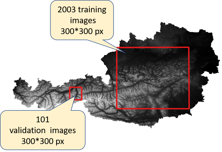
Fig. 2: Training and validation data for regions in Austria.
The data were downscaled with GDAL from 10 m to 30 m, using nearest neighbour interpolation, and then upsampled with cubic interpolation back to 30 m. The data can be downloaded here (under licence: Geoland.at (2020) Attribution 4.0 International, CC BY 4.0).
Update: Another 2001 training datasets could be downloaded here (under licence: Geoland.at (2020) Attribution 4.0 International, CC BY 4.0).
The pixel values in the training area have an uneven distribution (see below), which is not ideal for machine learning.
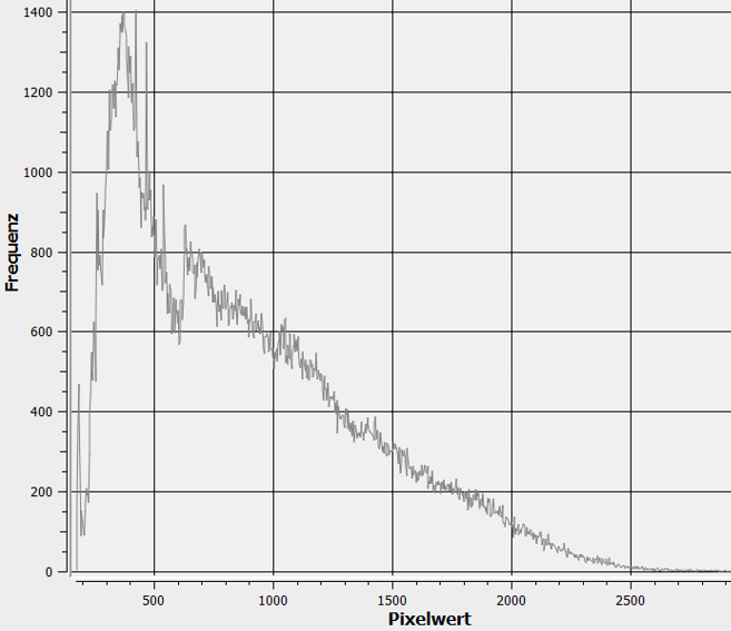
Fig. 3: Histogram of pixel values in the training area.
Types of Super-resolution algorithm
In general, SR techniques can be divided into two groups (see Figure 4 below):
1) those that give a high perceptual quality (i.e. the results look good to human beings)
2) those that give high accuracy (i.e. reasonable data values that are good for DEM processing)
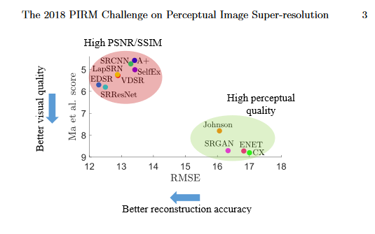
Fig. 4: Super-resolution algorithms, plotted according to the mean reconstruction accuracy (measured by RMSE values) and mean perceptual quality (source: Yochai Blau, Roey Mechrez and Radu Timofte - The 2018 PIRM Challenge on Perceptual Image Super-resolution)
For SR DEM, the second group is the right choice.
Previous attempts
- Enhanced Deep Residual Networks for Single Image Super-Resolution, implementation by Krasserm (Github)
- Enhanced Deep Residual Networks for Single Image Super-Resolution, implementation by Weber with OpenCV (Github)
- Image Super-Resolution Using Deep Convolutional Networks (SRCNN), implementation by Green (Github)
Unfortunately no better results could be achieved than with simple cubic upsampling.
Here is a tryout with Krasserm’s Super-Resolution EDSR. The algorithm needs an image with three layers (RGB). The usual procedure for greyscale images is simply to create a three-layer input with the same values. Finally, proceed the image with (band1 + band 2 + band3) / 3.
 |
 |
| Original resolution 10 m | Downsampling NN 30 m input |
 |
 |
| Cubic upsampling 10 m | EDSR 10 m |
Fig. 5: Comparison between the original 10 m dataset, the downsampled 30 m dataset and the derived products.
As can be seen from Fig. 5, the EDSR SR data looks sharper than the simple bicubic upsampling data, and is perhaps slightly too sharp. Statistics for the data are given below.
| Mean (abs) [m] | Max [m] | Min [m] | STDDEV [m] | |
| Original | 385.87 | 503.89 | 310.45 | 32.66 |
| Cubic Upsampling | 385.87 | 503.42 | 311.05 | 32.66 |
| SR Band 1 | 385.60 | 502.68 | 309.08 | 32.61 |
| SR Band 2 | 385.82 | 503.09 | 309.19 | 32.65 |
| SR Band 3 | 386.02 | 503.52 | 308.99 | 32.7 |
| SR (1+2+3)/3 | 385.81 | 503.07 | 309.08 | 32.65 |
| abs(original - derived) | ||||
| Cubic | 0.16 | 9.69 | 0 | 0.32 |
| SR Band1 | 0.35 | 13.01 | 0 | 0.35 |
| SR Band2 | 0.23 | 13.58 | 0 | 0.35 |
| SR Band3 | 0.25 | 13.53 | 0 | 0.35 |
| SR (1+2+3)/3 | 0.22 | 13.37 | 0 | 0.35 |
Tab. 2: Comparison of statistics for the processed data (for the test area shown in Figure 6)
The results in Table 2 show that with standard EDSR processing, no better results could be achieved than with ordinary cubic interpolation. Be aware that when using QGIS for comparison, the statistics obtained are only approximations. You can see this from the STATISTICS_APPROXIMATE=YES parameter. It is therefore better to use gdalinfo -stats for statistics.
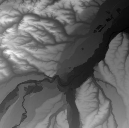
Fig. 6:Test area for the data shown in Table 2 (EPSG:31287, 435000.0, 460000.0 : 450000.0, 475000.0).
We will now look at a more mountainous region.
| Mean (abs) [m] | Max [m] | Min [m] | STDDEV [m] | |
| Original | 1244.13 | 2641.45 | 525.24 | 478.32 |
| Cubic Upsampling | 1244.13 | 2634.0 | 525.29 | 478.31 |
| SR Band 1 | 1243.86 | 2642.54 | 524.44 | 477.57 |
| SR Band 2 | 1244.06 | 2644.0 | 524.92 | 478.16 |
| SR Band 3 | 1244.2 | 2647.24 | 521.86 | 478.88 |
| SR (1+2+3)/3 | 1244.04 | 2644.59 | 523.74 | 478.2 |
| abs(original - derived) | ||||
| Cubic | 1.1 | 63.88 | 0 | 1.84 |
| SR Band1 | 1.51 | 64.37 | 0 | 2.02 |
| SR Band2 | 1.3 | 63.66 | 0 | 1.99 |
| SR Band3 | 1.4 | 61.14 | 0 | 2.0 |
| SR (1+2+3)/3 | 1.27 | 63.05 | 0 | 2.0 |
Tab. 3:Comparison of statistics for processed data (for the test area shown in Figure 7)
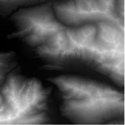
Fig. 7:Test area for the data shown in Table 3 (EPSG:31287, 130000.0, 360000.0 : 145000.0, 375000.0)
The results obtained by Müller et al. 2020 with different SR techniques also show that when applied to real data (satellite imagery in this case), cubic upsampling is hard to beat using standard SR techniques.
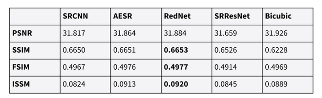
Tab. 4: Results of different super-resolution techniques compared to bicubic upsampling (Müller et al. 2020: “Super-resolution of Multispectral Satellite Images Using Convolutional Neural Networks”)
For an overview of SR techniques and metrics, have a look at the paper. The peak signal-to-noise ratio (PSNR) is defined by the mean squared error (MSE) and maximal possible value, and higher values are better.
VDSR-based super-resolution DEM
Very Deep Super Resolution (VDSR) CNN based on the implementation of George Seif.
An implementation of an SR CNN was proposed by Kim, Jiwon, Jung Kwon Lee, and Kyoung Mu Lee. "Accurate image super-resolution using very deep convolutional networks," Proceedings of the IEEE Conference on Computer Vision and Pattern Recognition, 2016.
More about convolution neural networks.
Code for DEM processing is available from Github:

This is a Jupyter Notebook project running on Google Colab with data storage on Google Drive. It could also be adapted to use local resources.
Slightly adapted model (4*4 filter kernel) of the original implementation.
Upscale Factor 3
Processing Epochs: 5250
Processing Time: ~ 200 hours
Carbon Footprint: ~ 25 kg CO2, compensation via Atmosfair.de.
Datasets: 2003 training and 101 validation datasets (each 300*300 px). See the Test data-section for download and licence.
Hyper Parameters: filters 64, kernel 4, adam 0.00001, conv2d layers 20
Results
| SR | Cubic | SR sliced | Cubic sliced | |
| MAE | 95 | 6 | 59 | 42 |
| RMSE | 101 | 0 | 101 | 0 |
| PSNR | 101 | 0 | 101 | 0 |
| SSIM | 80 | 21 | 79 | 22 |
Tab. 5: Comparison of the best results obtained for the metrics of mean absolute error (MAE), root mean squared error (RMSE), peak signal-to-noise ratio (PSNR) and structural similarity index (SSIM) for 101 validation datasets using VDSR and cubic upsampling. Datasets were sliced by 15 pixels to reduce border effects.
Overall, the RMSE for the validation dataset was improved by 2.04% (1.482 vs. 1.513), and the MAE was almost zero (0.8645 vs. 0.8640). Maximum error was improved by almost 0.5 m.
The landscape of the test area (Austria) is formed by fluvial and glacial erosion. Thus the model may not fit to other landscapes.
Update 5/2021: This model gave unacceptable results in a test with a fjord landscape in Scandinavia.
Tuning improved the results of the original model (see Keras Tuner section).
Hyper Parameters: filters 32, kernel 9, adam 0.0001, conv2d layers 11
Results after tuning
| SR | Cubic | SR sliced | Cubic sliced | |
| MAE | 101 | 0 | 101 | 0 |
| RMSE | 101 | 0 | 101 | 0 |
| PSNR | 101 | 0 | 101 | 0 |
| SSIM | 96 | 5 | 100 | 1 |
Tab. 5.1: Comparison (after tuning) of the best results obtained for the metrics of mean absolute error (MAE), root mean squared error (RMSE), peak signal-to-noise ratio (PSNR) and structural similarity index (SSIM) for 101 validation datasets using VDSR and cubic upsampling. Datasets were sliced by 15 pixels to reduce border effects.
Overall, the RMSE for the validation dataset was improved by 7% (1,407 vs. 1.513), and the MAE by 4.6% (0.824 vs. 0.864). Maximum error was improved by 0.8 m.
Doubling the training datasets halves the number of epochs, but did not result in better metrics in this case.
Statistics for the first ten validation datasets are given below.
| Validation dataset | SR MAE | Cubic MAE | SR RMSE | Cubic RMSE | Max. SR | Max Cubic |
| 278490_371780 | 0.746 | 0.761 | 1.152 | 1.208 | 15.358 | 16.734 |
| 293400_360980 | 1.205 | 1.242 | 2.323 | 2.440 | 59.126 | 60.862 |
| 275640_359420 | 0.658 | 0.691 | 1.151 | 1.253 | 21.883 | 23.278 |
| 282360_365720 | 0.754 | 0.810 | 1.165 | 1.281 | 17.505 | 18.204 |
| 278400_377660 | 0.648 | 0.700 | 1.013 | 1.136 | 12.220 | 11.460 |
| 280980_358340 | 1.425 | 1.5108 | 2.450 | 2.688 | 35.477 | 36.714 |
| 271440_374750 | 0.625 | 0.659 | 0.981 | 1.013 | 13.160 | 12.368 |
| 279090_369500 | 0.782 | 0.808 | 1.168 | 1.238 | 17.023 | 18.654 |
| 270780_357290 | 1.092 | 1.164 | 2.031 | 2.194 | 30.848 | 34.771 |
| 290100_367340 | 0.651 | 0.685 | 1.026 | 1.111 | 14.900 | 14.000 |
Tab. 6: Comparison of the basic statistics (mean absolute error, mean squared error, maximum error) for the first ten validation datasets
| Validation dataset | SR PSNR | Cubic PSNR | SR SSIM | Cubic SSIM |
| 278490_371780 | 68.74 | 68.328 | 0.993 | 0.993 |
| 293400_360980 | 62.643 | 62.219 | 0.989 | 0.988 |
| 275640_359420 | 68.742 | 68.007 | 0.991 | 0.990 |
| 282360_365720 | 68.637 | 67.812 | 0.994 | 0.993 |
| 278400_377660 | 69.857 | 68.856 | 0.994 | 0.992 |
| 280980_358340 | 62.008 | 61.379 | 0.992 | 0.991 |
| 271440_374750 | 70.654 | 69.858 | 0.994 | 0.993 |
| 279090_369500 | 68.617 | 68.109 | 0.991 | 0.990 |
| 270780_357290 | 63.810 | 63.140 | 0.992 | 0.991 |
| 290100_367340 | 68.742 | 69.051 | 0.995 | 0.994 |
Tab. 7: Further comparison of the metrics of peak signal noise ratio (PSNR) and structural similarity index (SSIM) for the first ten validation datasets (higher values are better).
The maximal value of the PSNR was set to the maximum value for the whole training region (3150 m).

Fig. 8: Border effects in a difference image (abs(original - superresolution).
Surprisingly was that the border effect for the cubic upsampling was even more relevant.
| MAE before | MAE after | Difference | |
| Super Resolution | 0.8229524 | 0.77234507 | 0.050607324 |
| Cubic Upsampling | 0.81898385 | 0.761203 | 0.05778086 |
Tab. 8: Metrics (mean absolute error) for super resolution and cubic upsampling, before and after slicing the border from 300*300 px to 270*270 px, for the first validation image (278490_371780).
It is important to slice the results to avoid these border effects through the filter by convolution neural networks (CNNs) and missing data at the edges in cubic upsampling. Although the use of padding may reduce the problem for CNNs, the effects are still present.
Watch the algorithm learning
Model Hyperparameters: filters 64, kernel 4, adam 0.00001, conv2d layers 20
2003 training datasets
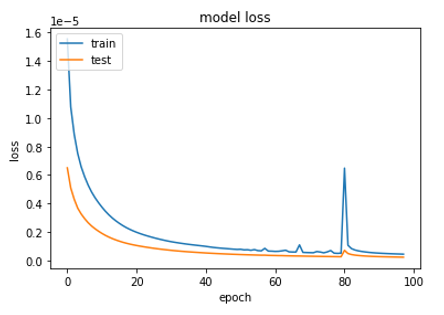
Fig. 9: Loss for epochs 5 to 100. The first five epochs were removed from the plot for clearer presentation.
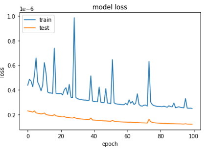
Fig. 10: Loss for epochs 100 to 200.
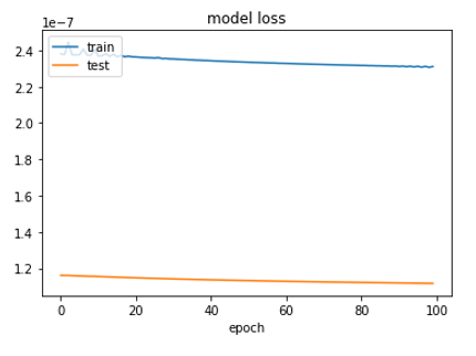
Fig. 11: Loss for epochs 300 to 400.
Update 17.2.2021: VDSR model with upscale factor 5
The retrieved hyperparameters with the Keras Tuner are identical with that of the upscale factor 3 model.
Processing time takes about 400 hours (15300 epochs).
The overall error is much bigger and the improvement is not as good as for the upscale 3 model. In some test areas the cubic upsampling is even better (see table 8 below).
Mean Absolute Error: 1.792 (cubic upsampling) vs. 1.74 (vdsr) ~ 2.94 % improvement.
Root Mean Square Error: 2.91 (cubic upsampling) vs. 2.78 (vdsr) ~ 4.51 % improvement.
| SR | Cubic | SR sliced | Cubic sliced | |
| MAE | 97 | 4 | 88 | 13 |
| RMSE | 101 | 0 | 95 | 6 |
| PSNR | 101 | 0 | 95 | 6 |
| SSIM | 84 | 17 | 83 | 18 |
Tab. 8: Comparison of the best results obtained for the metrics of mean absolute error (MAE), root mean squared error (RMSE), peak signal-to-noise ratio (PSNR) and structural similarity index (SSIM) for 101 validation datasets using VDSR and cubic upsampling with factor 5. Datasets were sliced by 15 pixels to reduce border effects.
Download upscale factor 5 test data - same as in the test data section, just with a different downscale factor. Under licence: Geoland.at (2020) Attribution 4.0 International, CC BY 4.0).
Weights Upscale factor 5 results - on GitHub.
Keras Tuner
The Keras Tuner is a library that helps you pick the optimal set of hyperparameters for your TensorFlow program.
The following Hyperparameters were adapted of the VDSR CNN:
- Filters values [4,8,16,32,64]
- Kernel size values [5,9,15,21]
- Learning rate adam values [0.001, 0.0001, 0.00001, 0.000001]
- number of Con2D layers range [1,30]
Only 100 training images were used with 50 epochs. It is important to use as many epochs till the model starts to converge.
The best score was reached with:
- Filters = 32
- Kernel size = 9
- Learning rate adam = 0.0001
- number of Con2D layers = 11
Of course this model was also much faster than the original VDSR model. But does this also scale up with thousands of training images and epochs?
| Model | MAE [cm] | RMSE [cm] |
| cubic upsampling | 0.864 | 1.513 |
| filters 64, kernel 4, adam 0.00001, conv2d layers 20 | 0.865 | 1.482 |
| filters 32, kernel 9, adam 0.0001, conv2d layers 20 | 0.834 | 1.416 |
| filters 32, kernel 9, adam 0.0001, conv2d layers 11 | 0.824 | 1.407 |
Tab. 10. Metrics (mean absolute error and root mean square error) for different hyper parameters compared to simple cubic upsampling (2003 training images, metrics after slicing).
It seems that way! Results in a faster and much better model, improving MAE by 4,63 % and RMSE by 7%. By comparison the metrics for the original model: MAE: -0.06%, RMSE = 2.04%
Next Steps
A Mean Absolute Error improvement of about 4.6 % compared to simple cubic upsampling is still not that impressive.
Other types of SR techniques such as Cycle-GANs and Pix2Pix seemed interesting. Anyway, at this time these unsupervised models are not better than the usual state of the art supervised models (Yuan Yuan et al.).
I played around a bit with the great deep learning library FastAI, but unfortunately didn't get convincing results. But try it yourself, here are some templates on GitHub: FastAI4DEM.
If an improvement of 10% is reached, the 50 m Bavarian DTM will be processed.
Publications and Implementations
Here is a great list of different SR implementations: Awesome Open Source - TOP Super Resolution Open Source Projects
List of some publicly available papers about SR with DEMs:
Bekir Z Demiray, Muhammed Sit and Ibrahim Demir - D-SRGAN: DEM Super-Resolution with GenerativeAdversarial Networks
Dongjoe Shin, Stephen Spittle - LoGSRN: Deep Super Resolution Network for Digital Elevation Model
Donglai Jiao et al. - Super-resolution reconstruction of a digital elevation model based on a deep residual network
Mohammad Pashaei et al. - Deep Learning-Based Single Image Super-Resolution:An Investigation for Dense Scene Reconstruction with UAS Photogrammetry
Yuan Yuan et al. - Unsupervised Image Super-Resolutionusing Cycle-in-Cycle Generative Adversarial Networks
Zherong Wu, Peifeng Ma - ESRGAN-BASED DEM SUPER-RESOLUTION FOR ENHANCED SLOPE DEFORMATION MONITORING IN LANTAU ISLAND OF HONG KONG