OpenDemEU Background

Update 2020
EVRF 2019 has brought a lot of changes.
The INSPIRE Data Specification on Elevation–Technical Guidelines defined that the EVRF2007 realization of EVRS should be adopted as height vertical reference for pan-European geo-information.
EVRF2019 points are now public available.
Download processed as Shape by OpenDEM
geopv & norm_h = zero tide
geop_v_1 & norm_h_1 = mean tide
With the Infrastructure for Spatial Information in the European Community (INSPIRE) more and more high resolution digital elevation models under free licenses are published.
The theme of elevation is part of the INSPIRE Annex 2. Unfortunately, the data are mostly only provided with national horizontal and vertical reference systems and an easy pan-European utilisation is not possible.
The aim of the project is to derive a pan-European digital terrain dataset with a standardised horizontal- and vertical reference system. Digital surface models are not recognised at this stage.
There are three derived products:
High-resolution projected tiles: In a 50*50 km raster as GeoTIFFs. The spatial reference system is the ETRS89 Lambert Azimuthal Equal-Area projection coordinate reference system (EPSG:3035) and vertical datum EVRS2000 (EPSG:5730). Resolutions below 1 m were recalculated to a 1 m DTM with a cubic resampling method to create manageable datasets below 10 GB.
1-arc second European geographic tiles: The typical SRTM style 1°*1° degree tiles with 1-arc second resolution as GeoTIFFs. The spatial reference system is geographic, lat/lon with horizontal datum ETRS89, ellipsoid GRS80 (EPSG:4258) and vertical datum EVRS2000 with geoid EGG08 (EPSG:5730).
1-arc second wgs84 geographic tiles & contours: The typical SRTM style 1°*1° degree tiles with 1-arc second and 3-arc second resolution as hgt. files. The .hgt files are 16bit integer format, so the height values are rounded to full metres. The spatial reference system is the world geodetic system 1984 (EPSG:4326) and vertical datum EVRS2000 with geoid EGG08 (EPSG:5730). Be aware that no epoch was used during transformation (see below) and therefore EPSG:4258 is the better choice. Anyway, wgs84 was the users choice to fit to the wide spread SRTM datasets. Additionally, contour lines as shape files are generated from the 3-arc seconds resolution tiles in the same manner as the global shape dataset was derived.
Background
High resolution DEMs involing complex problems that do not matter in low resolution DEMS like SRTM, ASTER & Co in which the RMS error is so big that any other problems are marginal.
PLEASE READ THE FOLLOWING INFORMATION CAREFULLY TO BE AWARE OF THE SIMPLIFIED PROCESSING STEPS!
Europe is on the move!
The European plate is shifting in general at about 3 cm in the northeast direction (see Fig. 1).
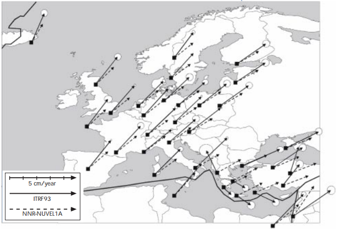
Fig.1: General northeast shift of the European plate in cm/a - compared to the plate motion models ITRF-93 and NNR-NUVEL 1A (source: European Commission, Joint Research Centre, Space Applications Institute Proceedings & Recommendations of Spatial Reference Workshop, November 1999)
Therefore the pan European reference system ETRS89 is an earth-fixed system in which the Eurasian plate as a whole is static. In 1989 ETRS89 was identical with WGS84 / ITRS. But since then, we have had an annual shift of about 3 cm to the northeast. To do a proper transformation the epoch has to be recognised. This does not matter with mass GPS receivers which have an accuracy far below this shift. But when you are using DGPS techniques or high-resolution DEMs take this into account.
We also have a post-glacial rebound (e.g. in Scandinavia) (see Fig. 2).
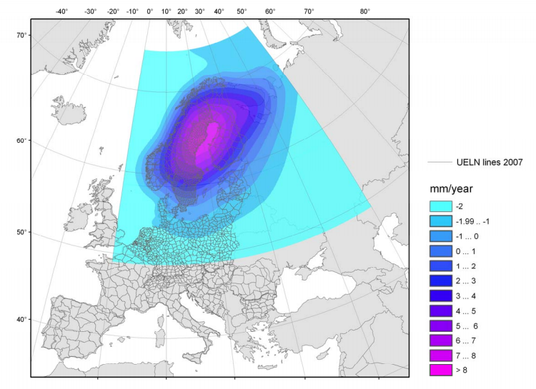
Fig. 2: Post-glacial rebound in Scandinavia (souce: Martina Sacher, Johannes Ihde, Gunter Liebsch - Das EVRF2007 als aktuelle Realisierung des europäischen Höhenreferenzsystems).
Thus, Europe is on the move in all directions, and this is hard to handle.
The pan European Vertical Reference System (EVRS) is also changing a lot, since more and more countries participate and national reference systems are updated. There is a separation between the definition of the EVRS and the realisation of a European Vertical Reference Frame (EVRF). As milestones, we have the systems EVRS2000 and EVRS2007.
Transformations of vertical datums
The transformation of vertical datums is trickier than the reprojection between two horizontal reference systems. Vertical transformations could be done, for example with gdaltransform (not with gdalwarp):
gdaltransform -s_srs EPSG:3035+5730 -t_srs EPSG:3035+5621 < in.xyz >out.xyz
The EPSG code consists of two parametres if you want to do a vertical transformation:
1. The horizontal reference system EPSG:3035, which is the ETRS89 Lambert Azimuthal Equal-Area projection coordinate reference system in this case.
2. The vertical datum, which is EPSG:5730 (EVRF2000) and EPSG:5621 (EVRF2007) in this case. Both are pan-European height reference systems.
The infile in.xyz contains the x,y,z coordinates:
4650012.500 1649987.500 332.763
4650037.500 1649987.500 337.635
4650062.500 1649987.500 342.153
4650087.500 1649987.500 347.179
4650112.500 1649987.500 352.244
If gdaltransform is executed, the outfile will look exactly the same as the input file. Why?
Both coordinate systems (horizontal and vertical) are correctly recognised. You can check them, for exapmle with testepsg 'EPSG:3035+5730', which is included in gdal.
To do a vertical transformation in gdal, you need a vertical shift grid, which is not yet available for EVRF2000 and EVRF2007. More information about vertical shift grids can be found on the VDATUM site of NOAA. For the USA, there many vertical shift grids available, that could be used with gdaltransform.
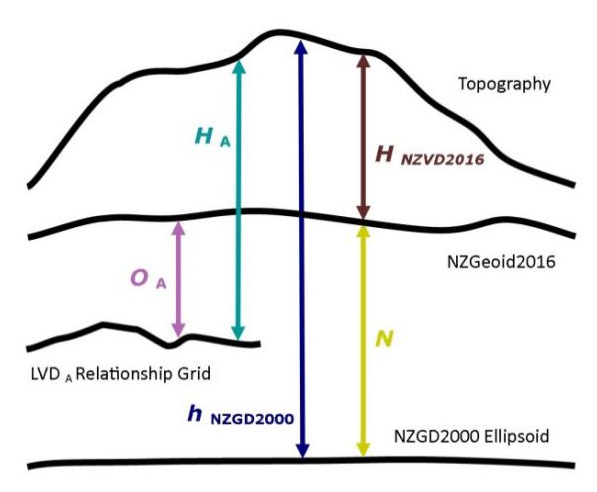
Fig. 3: Relationships between different height surfaces(source: Land Information New Zealand: Vertical Datum Relationship Grids).
| Symbol | Description |
| HNZVD2016 | NZVD2016 normal–orthometric height in metres |
| HA | LVD A normal–orthometric height in metres |
| HB | LVD B normal–orthometric height in metres |
| N | NZGeoid2016 value in metres at the NZGD2000 position of h (geoid height) |
| hNZGD2000 | NZGD2000 ellipsoidal height in metres |
| OA | The LVD A offset in metres evaluated from the relationship grid |
| OB | The LVD B offset in metres evaluated from the relationship grid |
The figure above is shows the relationship between different height surfaces. The ellipsoidal height is h. The Geoid Height is N. HNZVD2016 is the normal-orthometric height, which is H = h - N. The example is from New Zealand, where 13 local vertical datums (LVDs) are defined in terms of mean sea level at their respective standard ports. For each LVD there is a vertical datum relationship grid (LVD grid) in a 2’ x 2’ arc grid. The New Zealand Vertical Datum 2016 (NZVD2016) is defined by the NZGeoid2016 geoid. The vertical datum relationship grids can be used in conjunction with NZGeoid2016 to transform NZGD2000 ellipsoidal heights to normal-orthometric heights in terms of the local datums.
The relationship grids have been computed using the difference between normal-orthometric and ellipsoidal heights for GNSS-levelling marks within the LVD region (source).
Transformation between local datum and NZVD2016
The relationship grids (OA) transform NVDZ2016 height (H) from LVD height (HA): HA = H + OA (source).
When transforming between normal–orthometric heights in terms of LVD and NZVD2016 normal–orthometric heights, the following equations must be used:
HNZVD2016 = HA - OA
HA = HNZVD2016 + OA
Transformation between local vertical datums
When transforming normal–orthometric heights between different LVDs, the following equation must be used:HB = HA - OA + OB
Keep it simple...
At this point in time, shift grids in Europe are missing for EVRF2000 and EVRF2007 and also for the different national height systems. The only available pan-European DEM in EVRS is the EU-DEM. This is a Digital Surface Model with horizontal datum ETRS89, ellipsoid GRS80 and vertical datum EVRS2000 with geoid EGG08. SRTM & ASTER data were used by the Copernicus Project to derive the EU-DEM with a horizontal resolution of 1-arc second (~30 m).
UPDATE 1/2022: With EuroDEM a DTM is available with 2 ArcSeconds resolution.
The applied approach is simple. The EU-DEM serves as a base and and to the national height datasets were an offset applied as shown in Table 1 in the'Offset EVRF2000' column.
No proper transformation with a shift grid was applied, just an offset!
| Country | Reference Tide Gauge | Offset EVRF2000 [cm] |
Offset EVRF2007 [cm] |
Status | Comment |
| Albania | Durres | ||||
| Austria | Trieste | -35 | -34 | in progress | Metadata |
| Belgium | Ostend | -231 | -232 | ready | only Flanders |
| Belorussia | Kronstadt | 15 | |||
| Bosnia/Herzegovnia | Trieste | -34 | |||
| Bulgaria | Kronstadt | 15 | 23 | ||
| Croatia | Trieste | -33 | -31 | ||
| Czech Republic | Kronstadt | 11 | 13 | ||
| Denmark | 10 Danisg Tide gauges | 2 | 0 | ||
| England | 8 | 5 | |||
| Estonia | Kronstadt | 13 | 19 | ||
| Finland | Helsinki | 22 | -1 | ||
| France | Marseille | -49 | -47 | ||
| Germany | Amsterdam | 1 | 1 | ready | only NRW |
| Greece | |||||
| Hungary | Kronstadt | 14 | 14 | ||
| Iceland | no levelling heights | ||||
| Ireland | Malin Head | ||||
| Italy | Genoa | -35 | -28 | ||
| Lativa | Kronstadt | 10 | 15 | ||
| Lithuania | Kronstadt | 14 | 12 | ||
| Macedonia | |||||
| Moldavia | Kronstadt | 15 | |||
| Netherlands | Amsterdam | -1 | 2 | ready | Metadata |
| Norway | Tregde | 0 | -1 | ||
| Poland | Kronstadt | 16 | 17 | ||
| Portugal | Cascais | -32 | -25 | ||
| Romania | Constanta | 3 | 6 | ||
| Russia | Kronstadt | 15 | |||
| Slovakia | Kronstadt | 12 | 14 | ||
| Slovenia | Trieste | -33 | -39 | ready | Metadata |
| Spain | Alicante | -50 | -49 | ||
| Sweden | Amsterdam | 3 | -1 | ||
| Switzerland | Marseille | -35 | -23 | ||
| Turkey | Antalya | ||||
| Ukraine | Kronstadt | 15 | |||
| United Kingdom | Newlyn | 2 | |||
| Yugoslavia | Trieste |
Tab. 1: Differences between EVRF2000/2007 zero level and the zero levels of national height systems in cm (sources: Map Projections For Europe, EVRS website , Steps on the way to UELN05 and Enhancements of the web-based Geodetic Information and Service System).
For more information about the processing of the datasets, see the 'Meta' section of this topic.
Processing of the high resolution tiles
The following general processing was applied with GDAL 64 bit version:
1. Fill nodata areas when necessary with gdal_fillnodata.
2. Mosaic the national DTMs if necessary (gdalwarp).
3. Reproject the DTM mosaic to EPSG:3025 (gdalwarp).
4. Set the nulldata value to --32768 (gdalwarp).
5. Subset the DTM (gdalwarp).
6. Add or subtract the value from Table 1 with gdal_calc.
If necessary in border regions were the tile is not completely filled by the DTM:
7. Resample the EU-DEM to the desired resolution of the DTM (gdalwarp).
8. Mosaic the EU-DEM and the DTM (gdalwarp).
In border regions, different DTMs could also be merged with steps 5 and 6. The highest resolution in this case is always the reference.
Processing example in the border region of Belgium, the Netherlands and Germany
To test the quality of the processed tiles, overlapping areas in the border triangle were compared.
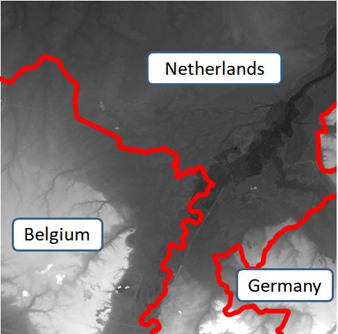
Fig. 4: Bordertriangle of Belgium, Germany and the Netherlands
| Belgium | Germany | Netherlands | |
| EPSG | 31370 | 25832 | 28992 |
EVRF 2000 Offset [cm] |
-231 | 1 | -1 |
| Resolution [m] | 1 | 1 | 0.5 |
Tab. 2: Basic data of the datasets
Table 2 shows the basic data of the compared datasets in the overlapping areas. For detailed information about the processing of the datasets see the OpenDemEurope --> Metadata section.
| Height in NRW (Germany) [m] | Height in Netherlands [m] | Absolute Difference [m] |
| 55.01 | 55.02 | 0.0005 |
| 61.05 | 60.88 | 0.17 |
| 68.72 | 68.61 | 0.11 |
| 63.34 | 63.31 | 0.03 |
| 74.1 | 74.07 | 0.03 |
| 32.15 | 32.08 | 0.07 |
| 35.47 | 35.39 | 0.08 |
| 36.57 | 36.69 | 0.12 |
| 45.52 | 45.47 | 0.05 |
| 30.99 | 31.1 | 0.11 |
| 49.12 | 49.33 | 0.21 |
| 93.82 | 93.73 | 0.09 |
| 58.11 | 57.92 | 0.19 |
| 110.18 | 110.04 | 0.14 |
| 51.43 | 51.38 | 0.05 |
| 40.68 | 40.55 | 0.13 |
| 44.86 | 44.82 | 0.04 |
| 42.05 | 41.94 | 0.11 |
| 37.19 | 37.08 | 0.11 |
| 63.51 | 63.45 | 0.06 |
| Mean difference [m] | 0.095025 | |
Tab. 3: Height difference at 20 test points after the processing in overlapping areas of NRW (Germany) and the Netherlands.
| Height in Flanders (Belgium) [m] | Height in Netherlands [m] | Absolute Difference [m] |
| 32.95 | 32.92 | 0.0015 |
| 62.79 | 62.78 | 0.0005 |
| 34.47 | 34.42 | 0.05 |
| 29.41 | 29.42 | 0.01 |
| 29.37 | 29.43 | 0.06 |
| 37.3 | 37.23 | 0.07 |
| 40.19 | 40.09 | 0.1 |
| 35.36 | 35.28 | 0.08 |
| 50.96 | 50.9 | 0.06 |
| 39.98 | 40.07 | 0.09 |
| 21.71 | 21.47 | 0.24 |
| 33.17 | 33.16 | 0.01 |
| 27.88 | 27.73 | 0.15 |
| 24.48 | 24.42 | 0.06 |
| 26.7 | 26.69 | 0.01 |
| 27.47 | 27.42 | 0.05 |
| 77.78 | 77.64 | 0.14 |
| 30.72 | 30.63 | 0.09 |
| 30.05 | 30.02 | 0.03 |
| 27.52 | 26.6 | 0.92 |
| Mean difference [m] | 0.1111 | |
Tab 4: Height difference at 20 test points after the processing in overlapping areas of Flanders (Belgium) and the Netherlands.
The overall difference of the measured heights in the overlapping areas was about one decimetre, with a maximum difference of about one metre.
Even if the correction was properly done, do not try to build a bridge on this dataset (no joke - for a rea- world example of what could happen due to incorrect calculation, see:: Rheintalbrücke 1984).
The richness of detail of the terrain structure in the derived 1-arc second products is obvious, even if the resolution is the same compared to the EU-DEM (see Fig. 5 and 6).
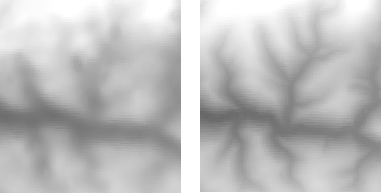
Fig. 5: Comparison of the EU-DGM (left) and the derived product on base of a high resolution DTM on the right (both 1-arc second resolution, region: subset of N51E007).
Processing of the EPSG:4258 geographic tiles
Resampling to EPSG:4258 with 3600 pixels (x,y) and the desired bbox, e.g.:
gdalwarp -ts 3600 3600 -s_srs EPSG:25832 -t_srs EPSG:4258 -te 7.0 51.0 8.0 52.0 -dstnodata "-32768" input.tif output.tif
Processing of the EPSG:4326 geographic tiles
The SRTM HGT format is somewhat special. The 3-arc second tiles, for example could be calculated with gdal_translate:
gdal_translate -of SRTMHGT -outsize 1201 1201 input_4258_n51e007.tif N51E007.HGT
which results in a bbox of:
xmin: 6.9995833333333337 xmax: 8.0004166666666663 ymin: 50.9995833333333337 xmax: 52.0004166666666663
For the 1-arc seconds tiles, 3601 * 3601 pixels are used. GDAL processes the bounding boxes automatically and converts the original float 32 dataset to a 16-bit integer dataset. Submetre values are therefore lost.
Also be aware that no epoch was used during transformation (see above).
GDAL processing tips and examples
Example fill nodata regions:
gdal_fillnodata -md 1000 -of GTiff unfilled.tif filled.tif
md= maxdistance in pixel
Example subset and reproject:
gdalwarp -s_srs EPSG:25832 -t_srs EPSG:3035 -te 4150000 3100000 4200000 3150000 -tr 1.0 1.0 -dstnodata "-32768" input.tif output.tif
s_srs = source reference t_srs = target reference te = bounding box of target file tr = x and y resolution dstnodata = no data value
Be aware that it is important to use the -tr parameter! Without this parameter gdalwarp in the example will produce an 49993 * 49993 image with a pixel size of 1.00014 m - even if the origin image has 5000 * 5000 cells and a pixel size of 1 m.
Mosaicing
The bottleneck while mosaicing with gdalwarp is the writing speed. It is much faster with a solid state drive (ssd).
The GDAL mosaicing tool gdal_merge reads all input datasets in memory and is not suitable for big datasets.
It is much faster to mosaic smaller regions and merge them afterwardswith gdalwarp. The mosaicing of 84 images took 1 hour and 35 minutes. After splitting, the calculation took 16 minutes:
gdalwarp nrw_280000_1 ... nrw_280000_14 1.tif gdalwarp nrw_284000_1 ... nrw_284000_14 2.tif gdalwarp nrw_288000_1 ... nrw_288000_14 3.tif gdalwarp nrw_292000_1 ... nrw_292000_14 4.tif gdalwarp nrw_296000_1 ... nrw_296000_14 5.tif gdalwarp nrw_300000_1 ... nrw_300000_14 6.tif gdalwarp 1.tif 2.tif 3.tif 4.tif 5.tif 6.tif all.tif
The last input image is rendered on top.
Raster calculation: subtract or add a value
gdal_calc -A input.tif --outfile= output.tif --calc=(A-0.01) --NoDataValue=--32768
In the example 1 cm is subtracted from the input height value. The calculation will not be applied at the no data value (-32768).
Raster calculation: handle multiple input null values
gdal_calc -A input.tif --outfile= output.tif --calc="A*(A!=9999)"
It is not possible to use gdalwarp with multiple source null values. In this example it is assumed that the null values of the input tiff are 0 and 9999. If the condition A!=9999 is false the value zero will be applied and the new pixel value is zero - a nice and quick way, thanks to this. Of course, this only works if one null value is zero. Also be aware of real zero values in your image.
Fill large areas of nodata values with real height values
Some areas were not covered by height data values by the data providers like the IJsselmeer in the Netherlands. These areas could be filled by real data values with GRASS r.null function, which is also available in QGIS. The processing of large nodata areas with gdal_fillnodata was not possible.
Add a specific value to a raster with a polygon layer
gdal_rasterize –l poly –burn 0 poly.shp raster.tif
The value 0 will be added to the tif in the area of the polygon.