Directional Cubic Convolution Interpolation
DEM resolution can be increased with Directional Convolution Interpolation
Content
Resampling & subpixel shift
Directional Cubic Convolution Interpolation (DCCI)
DCCI Faktor 2
DCCI Faktor 3
References
Resampling & subpixel shift
Downsampling with an even factor and nearest neighbours algorithm inevitably results in a subpixel shift.
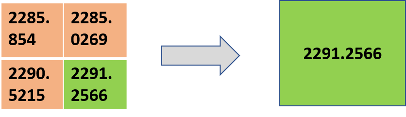
Fig. 1: Downsampling image values by factor 2 and nearest neighbours algorithm with GDAL
The widely distributed free software GDAL preserves the lower right pixel value as new image value in this case.
Following Upsampling with a cubic convolution and factor 2 results in new pixel values everywhere in the image (except the border pixels).
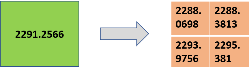
This results in a clearly recognisable in the upsampled image (see below).
Fig. 2: Pixel shift with gdalwarp: Original image vs. downsampling with nearest neighbour factor 2 and following upsampling with cubic convolution factor 2 (use mouse-over to see the effect).
Comparing 101 images (see test area) results in an overall mean average error of 2.62 metres. This is not the case with an uneven factor like 3. Original values are preserved, and overall mean average error for the test area and factor 3 was about 0.86 metres.
The subpixel shift problem and even resampling factors was solved by adding an empty row and column in first place (see DCCI Factor 2).
Fig. 3: Original image vs. downsampling with GDAL nearest neighbour factor 2 and following upsampling with DCCI factor 2 (use mouse-over to see the effect).
Datasets in figure 3 were sliced by 10 pixels to avoid border effects. It is clearly visible that the subpixel shift is reduced.
Directional Cubic Convolution Interpolation (DCCI)
Is an edge-directed image-zooming method, and an extension of the classical cubic convolution interpolation.
Original pixel values are preserved.
Original paper by D. Zhou1, X. Shen & W. Dong: Image zooming using directional cubic convolution interpolation
The implementation is based on Organa HQX implementation on GitHub.
DCCI Faktor 2
With this method, an accuracy of less than half a metre could be achieved with the test data (mean absolute error - MAE). Datasets were sliced by 10 pixels before comparison to reduce border effects.
The test data for factor 2 can be downloaded here (under licence: Geoland.at (2020) Attribution 4.0 International, CC BY 4.0).
The error in the standard procedure with GDAL cubic convolution upsampling of 2.62 metres (MAE) is mainly caused by the subpixel shift. Resampling with GDAL CC and factor 3 results only in an error of about 0.86 metres. Furthermore, this effect is only relevant at small resampling factors.
If the edge detection was ignored and only standard smoothing were used, the result was worse by about 7 % MAE (0.4843 vs 0.5229) compared to the best result (see table below).
| MAE [m] | T | K | |
| without edge detection | 0.52290 | - | - |
| proposed parameters | 0.55771 | 115 | 5 |
| best parameters | 0.48427 | 2310 | 1 |
Tab. 1: Metrics for mean absolute error (MAE) and varying DCCI thresholds (T) and exponents (K) for the test data.
In contrast to the original implementation with a proposed threshold T=115 and exponent K=5 a significantly higher threshold (2310) and significantly lower exponent (1) led to better results.
The optimal parameters for another dataset (25 images of 300*300 pixels) of a fjord landscape look very different.
| MAE [m] | T | K | |
| without edge detection | 0.20290 | - | - |
| proposed parameters | 0.17041 | 115 | 5 |
| best parameters | 0.16316 | 215 | 1 |
Here, an improvement of almost 20% could be achieved.
Tab. 2: Metrics for mean absolute error (MAE) and varying DCCI thresholds (T) and exponents (K) for a fjord landscape.
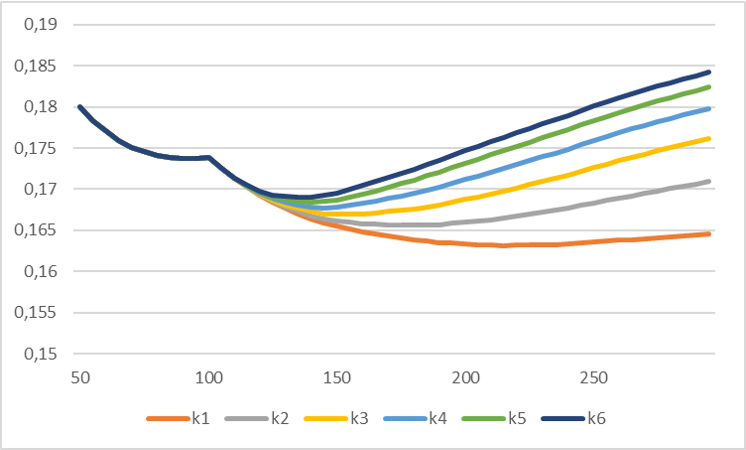
Fig. 4: Line chart of mean absolute error (y-axis, with comma delimiter) and thresholds T (x-axis) and varying Exponent K (coloured) for a fjord landscape.
Due to this large range of the parameters, it is not possible to determine the optimal parameters without reference data. With the estimator provided in the Jupyter Notebook below, the optimal parameters from reference data could be derived.
Another possibility could be an upstream downsampling of the input data, to derive the parameters which match best the scene structures of images.
| best results | test dataset1 | test dataset2 | ||||
| K | T | MAE [m] | T | K | MAE [m] | |
| factor 2 without edge detection | - | - | 0.52290 | - | - | 0.20290 |
| factor 2 proposed parameters | 5 | 115 | 0.55771 | 5 | 115 | 0.17041 |
| factor 2 DCCI | 1 | 2310 | 0.48427 | 215 | 1 | 0.16316 |
| factor 4 without edge detection | - | - | 2.61207 | - | - | 3.18295 |
| factor 4 proposed parameters | 5 | 115 | 1.41172 | 115 | 5 | 3.14568 |
| factor 4 dcci | 1 | 1300 | 1.31232 | 170 | 1 | 3.13768 |
| factor 2 dcci with 4er parameters | 1 | 1300 | 0.48429 | 170 | 1 | 0.16431 |
Tab 3: Comparison of the metrics of resampling with factor 2 and 4 for the two test datasets.
This method looks very promising; in both cases, accuracies of less than one centimetre were achieved compared to the optimal parameters.
The size of the image with the standard implementation is n -1. To prevent the subpixel shift, blank pixels were added at the beginning and top of the image. Slice the borders of your image after processing by 10 pixels to prevent border effects.
You could use GDAL gdal_translate with the srcwin parameter. This will cut the borders by 10 pixel of your 300*300 pixel image:
gdal_translate -srcwin 10 10 280 280 input.tif output.tif
Code of the DCCI4DEM Factor 2 is available on GitHub:

DCCI Faktor 3
In progress.
References
[1] D. Zhou1, X. Shen & W. Dong: Image zooming using directional cubic convolution interpolation