SRTM Processing
1. SRTM Digital Surface Model (DSM) Processing
2. SRTM Digital Terrain Model (DTM) Processing
If you want know what a DEM, DSM or DEM is, please visit the Definitions Section.
First the processing of an enhanced SRTM Digital Surface Model (DSM) is explained. This step is also necessary for the following processing of a Digital Terrain Model (DTM) on the basis of OpenStreetMap vector data. For detailed information see the Tutorial Section.
The Shuttle Radar Topography (SRTM) mission explored the structure of the earth surface in February 2000. The earth surface height was recorded between 60°N and 56°S. The data is available in 1*1 deegree (SRTM-1) for the USA and 3*3 degree (SRTM-3) tiles for the rest of the world. The resolution is for SRTM-3 three-arc-seconds, which is about 90 meters.
The SRTM data (Level 2.1, the most advanced processing state) can be downloaded at USGS.
1. SRTM Digital Surface Model (DSM) Processing
Due to the side-looking radar technique used by SRTM voids occur in mountainous regions as you see on Figure 1.
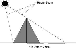
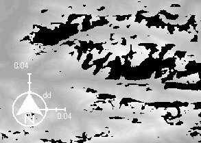
Fig.1: Voids resulting from side looking radar technique (left) and void pixels in the Alps are presented as black pixels (right).
These voids have the value "-32.768" and were filled with DEM data provided by Jonathan de Ferranti for the OpenDEM project. Many thanks for that. The data could be downloaded from the Viewfinders Panorama Homepage. Beside voids in mountainous regions, voids occur also near water bodies. A watermask was already applied for Level 2.1 SRTM data by the USGS (Link). These voids were filled by a 3*3 Matrix with the mean value (zero values were ignored). The process was performed 3 times inn order to eliminate all voids.
The data can be downloaded in the Download SRTM section under the Open Database License or CC-BY-SA License.
2. SRTM Digital Terrain Model (DTM) Processing
The SRTM mission mapped the structure of the earth´s surface including builtings and vegetation. OpenStreetMap data was used to correct the height values for forested and built up areas.
The resulting DTM is only an approximation, depending on many factors:
1. Time: The SRTM dataset is from February 2000 and many changes have occured since this time, especially in the built up regions
2. Quality of the OSM data: Completeness & accuracy
3. Accuracy of the SRTM dataset
4. Structure of the built up areas
5. Development stage and type of the forested areas
At first all land areas with zero values were set to a value of 1. This was done for a better visual discrimination between land and sea areas.
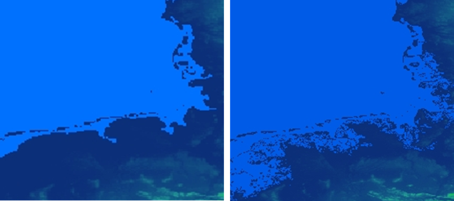
Fig. 2: Land values set to 1 (left) and the original dataset on the right for the German North Sea Coast (zeros in blue).
The OSM land tiles can be downloaded here. If the server is down, the data could also be downloaded from this server here (stamp 3/2010).
For the built up and forested areas a computed value was subtracted. The computation of the values is described in detail in the following
Built up areas are in general very heterogeneous. The question was: is itpossible to enhance the dataset by a subtracted constant value for the built up areas?
The following OSM tags were used to identify the built up areas:
highway: pedestrian
highway: residential
highway: living_street
man made:building
Forested areas should be not be as heterogeneous through as a more homogeneous canopy cover. But the recording of the data was in February. So in the northern hemisphere the structure of the forested areas was quite heterogeneous for the deciduous forests. The radar backscatter was reflected from the trunks and branches due to the absence of the leaves. Unfortunately, also for the coniferous forests the structure was not as homogeneous as expected.
The following OSM tags were was used to identify the forested areas:
natural: wood
landuse: forest
Whereas natural:wood is a tag used for natural woods the tag landuse:forest is used for forested woods. Please be aware that the usage varies from country to country.
The vector data was intersected with the SRTM raster data and two datasets were derived with the landuse classes of forest and urban. To compare these landuse classes with bare soils, also OSM vector data associated with moderate vegetation landuse:meadow and landuse:farm were intersected with the SRTM dataset.
Difference images from SRTM and an official 5 meter Digital Terrain Model were computed (vertical RMS error < 0.5 m). For the computation an Elevation Query Services (EQS) developed at the Department of Geoinformatics at the University of Heidelberg was used. The service calculates a local Triangulated Irregular Network (TIN) for the desired point coordinates. This is much more precise than just using a raster image for that purpose (Sorry,. the EQS is not available under a free software license).
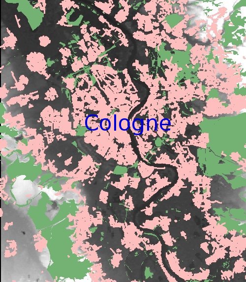
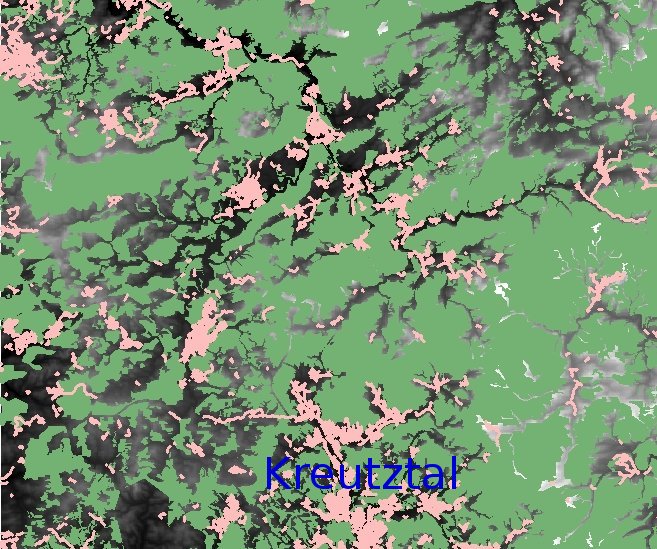
Three test areas in North-Rhine Westphalia where chosen, representing different landscapes and landuse characteristics (see Figure below, click image to enlarge it).
 |
|
 |
Cologne Region Flat Cologne-Bonn Bay with the greater Cologne urban area and surrounding rural areas |
Ruhr Basin Old metropolitan region with old coal mining areas and renaturalisation (54.579 Pixels). |
Rhineland Slate Mountains Forested mountainous area. (262.171 Pixels) |
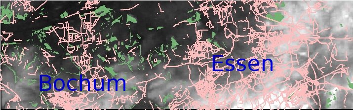
Fig. 3: built-Up areas were marked in pink and forested areas were marked in green (click to enlarge).
Have a look at the original data:
Table 1: Results of the computed difference images for the three test regions.
| Nr. | Difference Image: SRTM – DGM5 | Mean | Standard Deviation |
| Region Cologne | |||
| (1) | All (abs*) | 3.485 | 4.094 |
| (2) | Built Up | 2.548 | 2.362 |
| (3) | Built Up (abs) | 2.924 | 3.119 |
| (4) | Grassland/Farmland | 0.453 | 2.436 |
| (5) | Grassland/Farmland (abs) | 1.486 | 1.882 |
| (6) | Forest | 7.115 | 5.803 |
| (7) | Forest (abs) | 7.125 | 5.376 |
| (8) | Forest & Built Up areas (abs) | 4.405 | 4.362 |
| Ruhr Basin | |||
| (9) | All (abs*) | 2.750 | 2.653 |
| (10) | Built Up | 2.716 | 3.163 |
| (11) | Built Up (abs) | 3.283 | 2.570 |
| (12) | Grassland/Farmland | 0.143 | 1.232 |
| (13) | Grassland/Farmland (abs) | 3.033 | 2.608 |
| (14) | Forest | 2.511 | 4.379 |
| (15) | Forest (abs) | 3.770 | 3.356 |
| (16) | Forest & Built Up aereas (abs) | 3.397 | 2.780 |
| Rhenish Slate Mountains | |||
| (17) | All (abs*) | 10.433 | 8.521 |
| (18) | Built Up | 4.55 | 8.298 |
| (19) | Built Up (abs) | 5.934 | 7.372 |
| (20) | Grassland/Farmland | 3.934 | 7.438 |
| (21) | Grassland/Farmland (abs) | 6.164 | 5.762 |
| (22) | Forest | 11.674 | 10.255 |
| (23) | Forest (abs) | 12.671 | 8.699 |
| (24) | Built Up and Forest (abs) | 12.425 | 8.640 |
* abs: computed absolute mean values
The calculated absolute mean value for the areas associated with bare soils or spare vegetation was between +/- 0.5 meters ( Cologne Region) and +/- 6 meters in the Rhineland Slate Mountains. This fits to the studies from Czegka et. al. (2004) which derived an absolute vertical error of the SRTM dataset for Germany about +/- 2 meter to +/- 7 meters, depending on the surface structure.
For the associated built up areas the SRTM DSM dataset is in average about 2.5 meters higher than the official DTM for the Cologne Region and the Ruhr Basin. Depending on the relief the overestimation is higher for the Rhineland Slate Mountains.
The computed mean value for the associated forested areas was very different. Especially the mean value for the Ruhr Basin is, at about 2.5 meters very low. The forested areas in that region are in average quite small and errors due to georeferencing are more likely to affect small areas more greatly.
Margot Mayhofer (2007) estimated in her unpublished Master Thesis for the SRTM dataset (on the basis of CORINE landcover) an average RMS error for the forested areas of about 8-10 meters.
Forested Areas Correction
Table 2: Forested Areas Correction: Results of the computed difference images
| Nr. | Difference Image: SRTM – DGM5 | Mean | Standard Deviation |
| Region Cologne | |||
| (1) | Forest (Original Dataset) | 7.115 | 5.803 |
| (2) | Forest (Original Dataset) (abs) | 7.125 | 5.376 |
| (3) | Forest -7 meters | 4.695 | 3.536 |
| (4) | Forest Filter (max value) | 11.735 | 8.086 |
| (5) | Forest Filter (max value) - 12 meters (abs) | 5.696 | 5.702 |
| (6) | Forest Filter (max value) 2. pass | 14.814 | 10.290 |
| (7) | Forest Filter (max value) 2. pass - 15 m (abs) | 6.807 | 7.674 |
| (8) | Forest: 8 Neighbours | 8.499 | 5.584 |
| (9) | Forest: 8 Neighbours – 8 meters (abs) | 4.329 | 3.564 |
| Ruhr Basin | |||
| (10) | Forest (Original Dataset) | 2.511 | 4.379 |
| (11) | Forest (Original Dataset) (abs) | 3.770 | 3.356 |
| (12) | Forest: 8 Neighbours – 8 meters (abs) | 6.023 | 3.920 |
| Rhenish Slate Mountains | |||
| (13) | Forest (Original Dataset) | 11.674 | 10.255 |
| (14) | Forest (abs) | 12.671 | 8.699 |
| (15) | Forest -7 (abs) | 8.712 | 7.16 |
| (16) | Forest – 12 (abs) | 8.509 | 6.844 |
| (17) | Forest: 8 Neighbours – 8 meters (abs) | 8.664 | 7.157 |
For the Cologne Region a simple subtraction of the calculated mean value (3) results only in an error which was about 1/3 better than the original deviation (2). One explanation is the timeperiod of the data collection. In February the canopy cover of the deciduous forest is not homogeneous. The effect is also reported by Maryhofer (2007).The forest type is only sparsely tagged by the OSM community. Therefore the forest type could not be recognized by the correction.
Table 3: Mean Value and Standard Deviation of the SRTM data for different forest types in Austria with the 2-? Method (Mayrhofer 2007):
| Forest Type | Mean Value | Standard Deviation |
| Deciduous | 8.09 | 6.24 |
| Coniferous | 10.49 | 6.59 |
| Mixed | 10.13 | 6.93 |
To compute a closed canopy cover a 3*3 Matrix were used to calculate the maximal value within the matrix for the pixel (4). After that the resulting deviation was subtracted (5). Also a second pass was tried (6 & 7). The results were not as good as the simple subtraction (3). Especially on the edges of the forested areas the error increases through the applied intersection processing and georeferencing errors. To avoid that only the forest pixels were used which have also 8 Neighbours, which are classified as forest. For that pixels the deviation decreases (8) and the resulting subtraction is better than the original subtraction (7). The overall enhancement does not look very impressive at a first glance, but when you have a look at the histograms this makes much more sense.
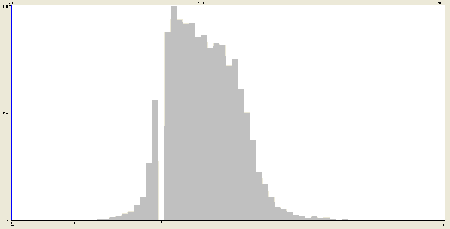

Fig. 4: Histograms of the difference images for the forested areas of the Cologne Region before (left) and after the correction (right) - click to enlarge.
The centre of the normal distribution is shifted to zero with the correction. The zero values are not included in the histograms and the calculated mean values (red line) are scaled in the visualisation to integer values which gives a wrong picture at the first glance. Nevertheless the distribution of the values is obviously better and no further work was done regarding adjustment.
The forested areas of the Ruhr Basin are very special. In this region renaturalisation of the old mining areas are wide spread as you see in the following Figure.

Fig. 5: Renaturalisation of mining areas in the Ruhr Basin. Potlatch Screenshot. Aerial Image (c) by YAHOO!
The height of the young trees is in fact very low. In 2000 perhaps there would not be trees anyway. The resulting deviation is in this case even more worse than the original data values. Nevertheless developing forested areas with low trees are usually only a small percentage of the total forested area.
The third case was the forest in the Rhineland Slate Mountains. In this mountainious area the difference image for the bare soils and grasslands differs for about 4 meters (Table 1 (20)). This is much more than in the other regions. This difference increases also for the forested areas. Astonishingly the results of the absolute difference images for the parameters -7 meters (15). -8 meters (17) and -12 meters (16) were almost the same.
In general the correction of the forested areas with a simple subtraction makes sense, but regionally the deviation could be even greater than in the original dataset. The following factors affect the results:
- development state
- forest type
- relief
built Up Areas Correction
Table 4: built Up Areas Correction: Results of the computed difference images
| Nr. | Difference Image: SRTM – DGM5 | Mean | Standard Deviation |
| Cologne Region | |||
| (1) | Built Up | 2.548 | 2.362 |
| (2) | Built Up (abs) | 2.924 | 3.119 |
| (3) | Built Up Filter Minimum (3*3) | 2.734 | 2.776 |
| (4) | Built Up: -3 meters (abs) | 2.215 | 2.242 |
| (5) | Built Up: -2 meters (abs) | 2.088 | 2.380 |
| (6) | Built Up: -1 meter (abs) | 2.343 | 2.575 |
| (7) | Built Up: 8 Neighbours | 2.541 | 2.541 |
| (8) | Built Up: 7 Neighbours | 2.438 | 3.619 |
| (9) | Built Up: 6 Neighbours | 2.579 | 4.123 |
| (10) | Built Up: 5 Neighbours | 2.624 | 4.075 |
| (11) | Built Up: 4 Neighbours | 2.593 | 4.512 |
| (12) | Built Up: 3 Neighbours | 2.686 | 5.683 |
| (13) | Built Up: 2 Neighbours | 4.179 | 5.683 |
| (14) | Built Up: 1 & 0 Neighbours | < 50 Pixels | |
| (15) | Built Up: 8 Neighbours -3 meters (abs) | 1.839 | 1.812 |
| (16) | Built Up: 8 Neighbours -2 meters (abs) | 1.758 | 1.913 |
| (17) | Built Up: 8 Neighbours with focal min | 2.007 | 2.345 |
| (18) | Built Up: 8 N. with focal min + 1 SRTM | 1.244 | 3.077 |
| Ruhr Basin | |||
| (19) | Built Up | 2.716 | 3.163 |
| (20) | Built Up (abs) | 3.283 | 2.570 |
| (21) | Built Up -3 meters (abs) | 2.280 | 2.195 |
| (23) | Built Up: -2 meters (abs) | 2.906 | 2.667 |
| (24) | Built Up: 8 Neighbours | 3.218 | 3.145 |
| (25) | Built Up: 7 Neighbours | 2.886 | 3.198 |
| (26) | Built Up: 6 Neighbours | 2.761 | 3.145 |
| (27) | Built Up: 5 Neighbours | 2.529 | 3.307 |
| (28) | Built Up: 4 Neighbours | 2.293 | 2.850 |
| (29) | Built Up: 3 Neighbours | 2.181 | 3.078 |
| (30) | Built Up: 2 Neighbours | 2.109 | 3.049 |
| (31) | Built Up: 1 Neighbours | 1.896 | 2.976 |
| (32) | Built Up: 8 Neighbours -3 meters (abs) | 2.241 | 2.216 |
| (33) | Built Up: 8 Neighbours focal min (abs) | 2.929 | 2.769 |
| (34) | Built Up: 8 N. with focal min + 1 SRTM | 3.166 | 2.840 |
| Rhinland Slate Mountains | |||
| (35) | Built Up | 4.55 | 8.298 |
| (36) | Built Up (abs) | 5.934 | 7.372 |
| (37) | Built Up -3 meters (abs) | 4.843 | 6.915 |
| (38) | Built Up -2 meters (abs) | 4.955 | 5.195 |
| (39) | Built Up: 8 Neighbours | 3.738 | 5.138 |
| (40) | Built Up: 7 Neighbours | 3.273 | 5.155 |
| (41) | Built Up: 6 Neighbours | 3.741 | 8.471 |
| (42) | Built Up: 5 Neighbours | 4.280 | 7.788 |
| (43) | Built Up: 4 Neighbours | 4.507 | 7.108 |
| (44) | Built Up: 3 Neighbours | 5.156 | 8.722 |
| (45) | Built Up: 2 Neighbours | 5.995 | 11.656 |
| (46) | Built Up: 1 Neighbours | 5.672 | 8.127 |
| (47) | Built Up: 0 Neighbours | < 50 Neighbours | |
| (48) | Built Up: 8 Neighbours -3 meters (abs) | 3.868 | 3.459 |
| (49) | Built Up: 8 Neighbours focal min (abs) | 5.598 | 6.58 |
| (50) | Built Up: 8 N. with focal min + 1 SRTM | 6.429 | 5.244 |
The first try for correction was a filter with a 3*3 Matrix, which computed the minimum value as the result (3). The assumption was that in the heterogeneous structure of built up areas always bare surface pixels could be found. Nevertheless a simple subtraction seems more effective with the subtraction parameters three, two and even one meter (4,5,6). Strong negative deviations seem to occur at the edges of the built up structures.
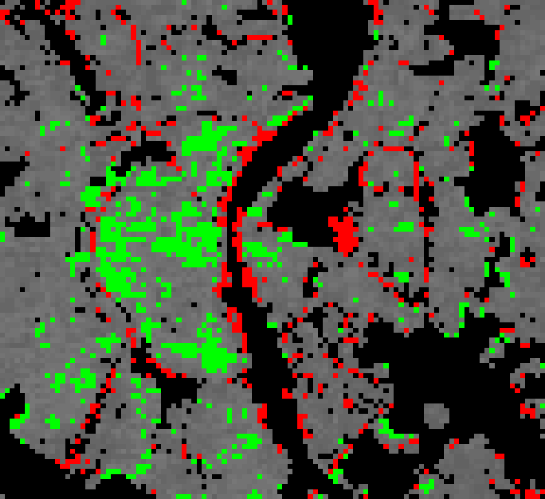
Fig. 6: City of Cologne- absolute difference image – 3 meters (4) with deviations greater than 3 meters in green and less than -3 meters in red (click to enlage)).
One reason for the deviations observed is the intersection processing. Also if only a small part of a vector is covering the raster cell, the whole raster cell will be mapped as a built up area. To avoid this deviations a kind of urban index was tested. All built up pixels were set to 1. Afterwards a focal analysis with the computation of the sum was applied (3*3 matrix, zeros were ignored). The resulting difference images show that also for the pixels with less than 4 neighbours (Tabl 4: 12-13, 29-31, 44-46) the value was in average not much lower than for the pixels with more than 5 neighbours (Tab. 4: 6-8, 23-25, 38-40). In the case of the Cologne Region and the Rhineland Slate Mountains the opposite was the case.
But for all three regions the best result was when the subtraction was applied only to the pixels with 8 neighbours (Table 4: 15, 32, 48). But because all other pixels with less than 8 neighbours show in average also positive deviations of about 3 meters, no focal filtering were applied in the end.
Another try was to compute a focal minimum (3*3 matrix) for all pixels with 8 neighbours (Table 4: 17, 33, 49). But the result was not better than the simple subtraction. Because it seems that that method leads to an underestimation of the height. 1 meter was added to the SRTM data before the computing of the difference images (Table 4: 18, 34, 50). The result for the Cologne Region was good (Table 4: 18), but not for the other test sites (Table 4: 34, 50).
The simple subtraction of 3 meters for all built up pixels results in an improvement of the absolute mean values from about 20 % (Rhineland Slate Mountains) to 30 % (Ruhr Basin). Again this is not a very impressive percentage but the following figures show that the centre of the distribution is shifted near to zero, as it should be.
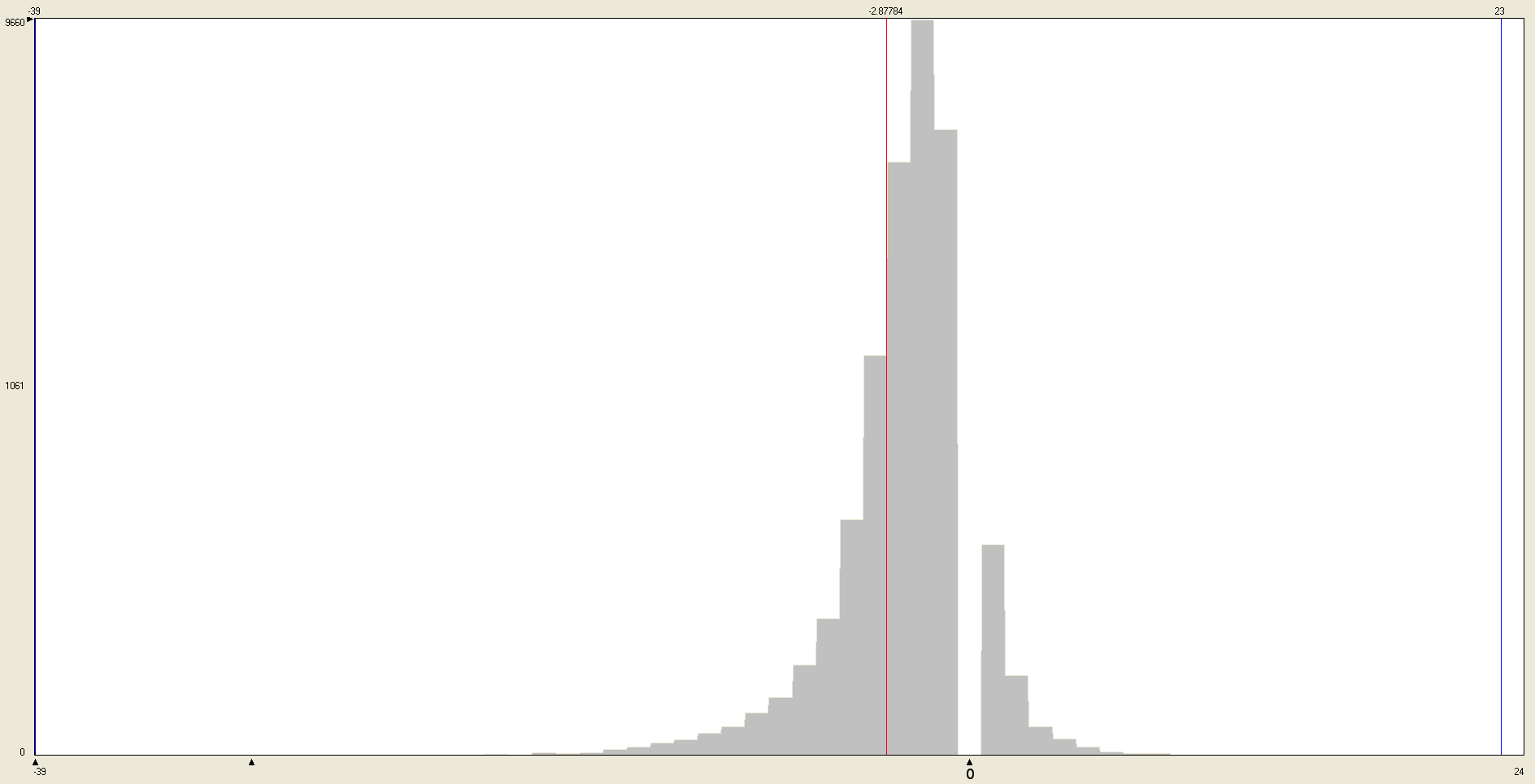
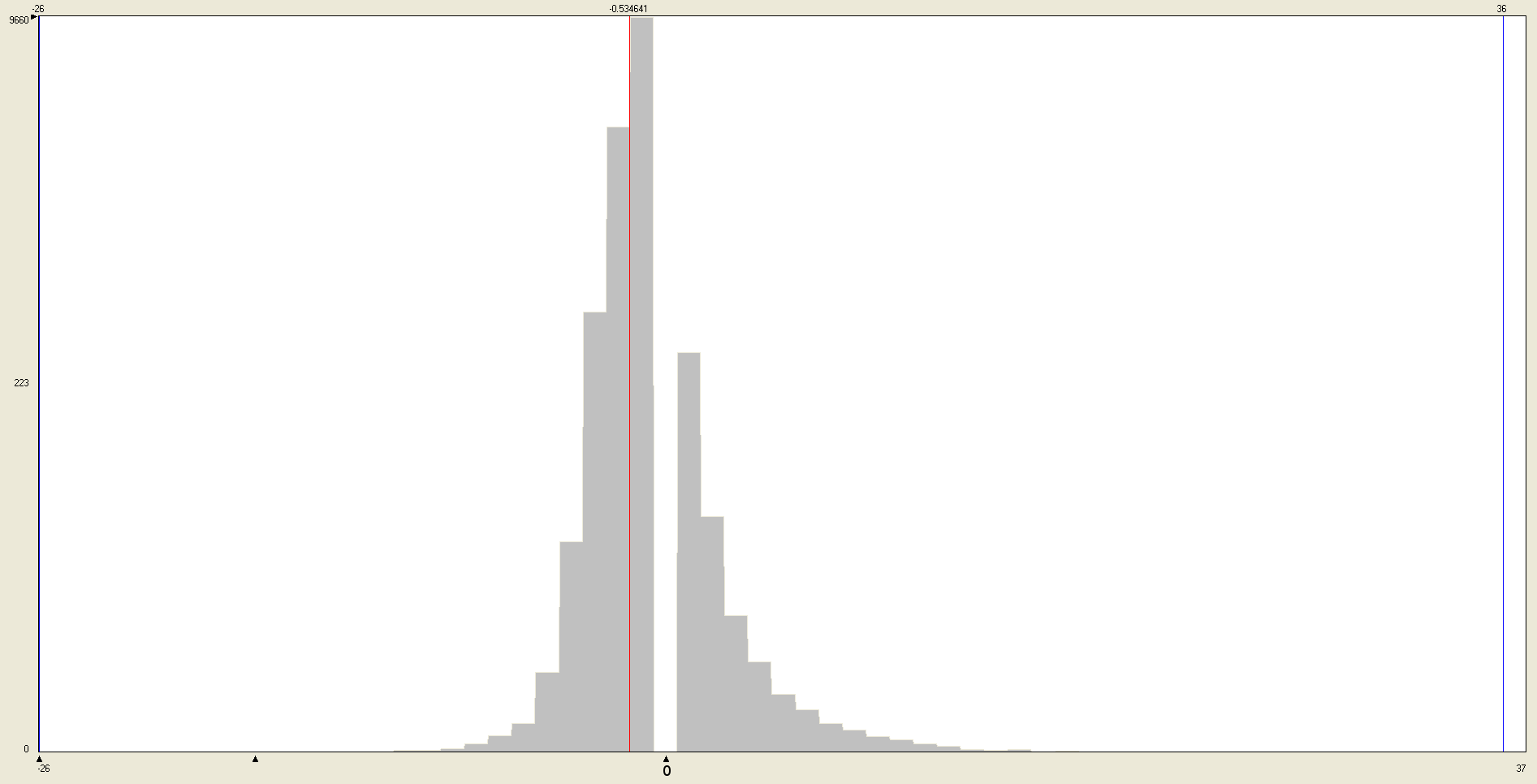
Fig. 7: Histograms of the difference images for the built up areas of the Region Cologne before (left) and after the correction (right) - click to enlarge.
Table 5: Results of the computed original and corrected absolute difference images for the three test regions.
| Nr. | Difference Image: SRTM – DGM5 | Mean | Standard Deviation | Histogram* |
| Region Cologne | ||||
| (1) | Forest/Built Up areas original (abs) | 4.405 | 4.362 | |
| (2) | Forest/Built Up areas corrected (abs) | 2.636 | 2.716 | |
| (3) | Grassland/Farmland (abs) | 1.486 | 1.882 | |
| (4) | All original (abs) | 3.485 | 4.094 | |
| (5) | All corrected (abs) | 2.597 | 3.122 | |
| Ruhr Basin | ||||
| (6) | Forest/Built Up areas original (abs) | 3.397 | 2.780 | |
| (7) | Forest/Built Up areas corrected (abs) | 2.683 | 2.141 | |
| (8) | Grassland/Farmland (abs) | 3.033 | 2.608 | |
| (9) | All original (abs) | 2.750 | 2.653 | |
| (10) | All corrected (abs) | 2.251 | 2.802 | |
| Rhenish Slate Mountains | ||||
| (11) | Forest/Built Up areas original (abs) | 12.425 | 8.640 | |
| (12) | Forest/Built Up areas corrected (abs) | 8.292 | 7.046 | |
| (13) | Grassland/Farmland (abs) | 6.164 | 5.762 | |
| (14) | All original (abs) | 10.433 | 8.521 | |
| (15) | All corrected (abs) | 8.043 | 7.141 | |
* Click to enlarge, for the histogramms of course no absolute values were used.
It could occur that the forested and built up areas overlap. In this case it was slightly better to overlap the forested areas over the built up areas (Cologne Region 2.636 vs. 2.661 and Rhineland Slate Mountains 7.046 vs. 7.015). The Ruhr Basin is an exception anyway due to the newly forested areas.
The processing was partly done with proprietary software at the Cartography Research Group of the University of Bonn. The research team around Prof. Dr. Zipf is now located at the University of Heidelberg (GIScience). The processed data is available under the actual OSM license (CC-BY-SA) at the Download SRTM Section.
A tutorial for the processing with free software is under development (Tutorial Section).
Literature
Czegka, W.. Behrends, K. & Braune, S. (2004). Die Qualität der SRTM-90m Höhendaten und ihre Verwendbarkeit in GIS. 24. Wissenschaftlich-Technische Tagung der DGPF. 15.-17.9.2004 Halle.
Mayrhofer. M. (2007): Erstellung eines Geländemodells für Mitteleuropa unter der Verwendung eines globalen Oberflächenmodells (SRTM), eines regionalen Geländemodells und eines überregionalen Landbedeckungsmodells (Corine Landcover 2000). Unpublished Master Thesis. Graz University of Technology. Austia.